Studies of statistics help to accurately model and make sense of research by combining logical rules and quantifiable, objective numerical data. While observations of most things may be easily converted into pure numbers, spotting and understanding clear patterns, trends, and meaning in those abstract, representational values may prove difficult. Statistics help eliminate noise and reveal hidden connections, informing us to make better decisions and predictions for the future.
Definition: Statistics
Statistics are used to collect, understand, and interpret data. A statistical analysis may be defined as reaching conclusions from quantitative data that may not be immediately obvious from raw, isolated numbers. This analysis is then applied to inform crucial decisions relating to an exploratory question.1
The steps, rules, and formulae capable of collecting, interpreting, and querying vast sets were developed to the point that all professional studies will still follow a rough version of the five-step methodology.
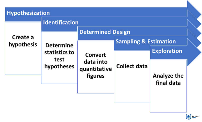
The 5 steps to analyzing statistics:
- Hypothecation: Also known as a hypothesis and functions as a theoretical statement that usually predicts a state of affairs or how subject A correlates to event B.
- Identification: Determining needed statistics to test the hypothesis and how each data set should be collected from each population. Filtering data that is too vague, unrepeatable, or unethical. Evaluating whether the data will change over time – or in different contexts, and whether the data is inferable.
- Determined Design: Planning how ‘raw’ data will be converted into quantitative figures, processed, and displayed. For this, select and describe relevant statistics. Identifying a population subsample.
- Sampling and Estimation: Collecting, collating, and processing data.
- Exploration: Systematically examining the final data for insights and testing for correlations. Data may be cross-referenced with other studies to establish a broader context.

Descriptive vs. inferential statistics
We commonly use two main types of ‘finished’ statistics – descriptive statistics and inferential statistics. Which category they match with depends on how, why, and where they are used and displayed.
| Type of statistics | Function |
| Descriptive statistics | • Seek to give readers an accurate, objective, numerical-format snapshot of a subject within a point or context. • are straightforward statements of revealed fact.2 • string together to produce longitudinal bar charts, line graphs, and pie charts illustrating a point by charting integer or percentage measurements over time.3 • can be safely published while highly uncertain.2 |
| Inferential statistics | • determine the repeating relationships within sets of descriptive statistics in order to model and make predictions. • help us set realistic expectations with a decent-sized sample.4 • the probability of a select common variable or outlier of statistics is highly predictable and thus inferable.2 |
Testing effects vs. correlations in statistics
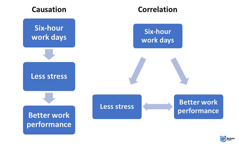
There are two common ways of analyzing statistics. These approaches relate to how we demonstrate correlation vs. causation in a population.
In a correlational study, a statistical hypothesis is tested to determine whether a proposed relationship between two variables is supported. A successful analysis might show that if variable A increases or decreases by X, variable B predictably increases or decreases by X as well.
However, correlation does not automatically imply causation. Completely unrelated variables may appear strongly correlated by chance — a spurious correlation. Rare or unusual datasets may create misleading patterns, or a third unseen variable Z may be responsible for connecting two factors that appear to correlate.
In contrast, a causative study evaluates whether X directly affects Y (positive causation) or whether a third-party factor, a confounding variable Z, is influencing the relationship. Causation analysis typically compares a control dataset (X = absent) with datasets where X is present. If Y shows no consistent, repeatable response to X, then the effect is considered non-causal.
These two approaches may also appear together in hybrid research designs. If X and Y correlate and each seems to influence the other’s behavior, a directional or cross-lagged analysis can help determine which variable has the stronger influence.

1. Determining the hypothesis in statistics
At the very start of every study based on statistics is a central theoretical proposition known as a hypothesis.
A hypothesis is a scientific question that briefly sets out the (dis)provable theory and the goals behind the study. It details the evidence of the statistics that need to be proven or disproven, or correlations and behavior in a set population investigated. The hypothesis itself is usually phrased as formulaic statistics (e.g., p = 0.05).
Relational studies seek to (dis)prove hypothetical effects, while casual studies seek to (dis)prove correlations. More than one hypothesis may be created in one research, where each may counter, confirm, or enhance our understanding of a previous hypothesis already tested and (dis)proven.
Null vs. alternative hypothesis
Every hypothesis comes in two parts.
The alternative hypothesis is the part that challenges our existing assumptions about a topic. It argues that a new proposition is true. Each alternative proposition comes complete with a polar opposite – a null hypothesis.
| Hypothesis | Function |
| Alternative hypothesis | • expresses broad casual statements of expected fact or as expected relational correlations. • expects qualitative statements that may also give additional context to the study. |
| Null hypothesis | • derives from the current, consensual 'status quo' answer to each study's central question(s). • gives outside context by establishing the state of research • offers authors a valid route to completion in the event of failure.7 |
If no contextual ‘common-sense answer is available, a counter-proposal may be invented by logically inverting the alternative (e.g. n = 1) or suggesting a random correlation (e.g. n = 0.05).
Frequentist vs. Bayesian statistics
When researching an exploratory hypothesis, a framework approach that gives the best chance of generating accurate statistical insights may be most relevant. Here are two philosophies that may help.
Thought experiment:
If a coin flips and the outcome is hidden, the probability of it being what it is, is still, logically, 100%. No known method can objectively and fairly predict what side the coin is lying on before revelation.
| Type of statistics | Function |
| Frequentist Statistics | • interpret open-endedly, making them suited to proving the alternative. • rely on direct, empirical evidence to quantify what's happening. • seek to discover statistical knowledge as it comes. |
| Bayesian Statistics | • rely on probability models that assume that hidden, absolute rules govern the data around us. • gather enough data on past events to enhance our understanding of the future with odds. • great for validating null hypotheses with strong background evidence • examine events and correlations within fixed, predictable systems. • are fundamentally conservative, assuming events don't change much.8 |
A fanatical frequentist would assume that every statistical value generated and gathered is random and absolute, with no known preconditions. In terms of the thought experiment, the coin is immeasurable until the palm opens.
A Bayesian may predict a reasonable 49.99% chance that the coin is on heads by using a parameter estimator. In relation to the thought experiment, the odds of a two-outcome scenario are so likely that an educated guess is worthwhile and informative.
Determining the research design in statistics
The research design is a short document detailing how a study will be structured and verify relevant data. It also outlines the methods and concepts used for analyzing the sampled statistics.
| Research design | Function |
| Correlational studies | • explore relationships between variables. • use direct comparison and mean regression graphing to assess whether the points affect each other and to what degree. • are used to further study or double-check past research of statistics |
| Descriptive studies | • aim to produce high-quality, descriptive statistics without any further analysis. • examine population factor presence, volume, and percentage frequency. • are a staple of market research and are often used to empirically inform less objective fields. |
| Experimental plans | • are more open-ended and deep ranging. • independently look at whether multiple unknown factors have any effect on each other. • explore new or obscure areas and establish confounding causative variables. |
Group level vs. individual level in statistics
In a study of statistics, determine whether participants should be compared as a group, individually, or mixed:
Between-subject design: Participant groups from the same population, unknowingly experience different tests. One group is designated as a ‘true’ control to create a basic frame of reference.
Within-subject design: All study participants experience one identical test scenario as one group with one set of sampling criteria. Participants are selected as randomly as possible to ensure no bias.
Mixed design: A combination of the above methods. While a mixed experimental study may still have one large group to test, two or more causative factors can be altered in repeated testing to make it a factorial study.
Measuring variables in statistics
Operationalization helps construct the skeleton of your final statistics model. Setting variable categories and methodology early on helps keep consistency in your measurements.
| Type of measurement | Function |
| Quantitative measurements | • sample numerical integers and percentages 'as is' (with rounding). • are excellent for precisely recording amounts of things and occurrences as n values. • Correlative values (e.g. R) express as quantitative. Example: Create a measurement by quantitatively describing that exactly 10 study participants were aged 18. While dry and objective, quantitative values can convey factual information to researchers and readers without expectations or implications. |
| Categorical measurements | • act like labeled boxes to fit diverse results into descriptive streams. • are practical tools that simplify complex, subjective, qualitative data into malleable 'at-a-glance' values by using set variable ranges. Example: Set up an absorbent categorical variable labeled 'Young' that collects all study participants aged 18-25. The combined n value created gives readers a quicker, qualitative judgement. |
2. Collecting data in statistics
Repeatable tests, and chosen populations to collect data from, are vital in analyzing empirical statistics. Moreover, deciding whether it’s appropriate to deliberately bias your sample population or groups and making sure your sample size is large enough to have scalable, real-world validity.
Sampling in statistics
It’s impractical, and expensive, to sample millions of independent values to get a reliable result. Therefore, investigating a representative wedge of what you want to study, is the more plausible option.
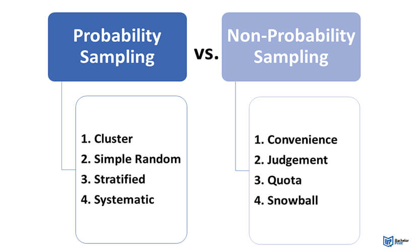
Extracting poll samples will accurately map how their million-strong source population is behaving. You may pick from two distinct methods for this:
| Probability sampling | Non-probability sampling |
| • all data points (e.g. person, node, recorded outcome) have an equal chance of being selected • Researchers determine who and what they draw from • Efficient enough for highly generalizable hypotheses and repeatable systems • Homogeneous, predictable populations may be described • Outliers, irreplicable results, warped percentages, and false positives may occur if applied too broadly |
• Participants are selected by category division or voluntary • Avoiding random chance allows researchers to focus on specific sub-sections • General inference is weaker, the applicability of the research to distinct areas is enhanced • Causative bias might result from advertising for enthusiastic participants. |

Sizes and procedures in statistics
To work out a representative sample size, use an online calculator. These will automatically give you a rounded figure representing the population within a 95% degree of accuracy via a short, complex formula.
Gathering the following additional technical estimates may also be essential:
Effect size: This represents the best guess at the strength of the effect that is in evaluation. For this, past studies and statistics, pilot studies, and informed guesswork may help create your reasonable estimate.
Population standard deviation: Defines how clustered and homogeneous the base population is on a numerical scale, expressed as an integer compared to past studies of the researcher.
Significance (alpha): Even the best statistical sets risk creating false conclusions about the null hypothesis due to random outliers. However, larger samples vastly reduce the chance of that happening. The Alpha value is usually set at 0.05, giving researchers a 1/20 chance of generating an unrepresentative set.
Statistical power: Depicts the best guess at the study’s probable chance of proving or disproving the null hypothesis. Power is typically above a minimum of 0.8 (80%).
If a sample population figure via calculation can’t be reached, a sample from a recent similar statistical study may be used instead. This technique may also help test a past study’s repeatability.
3. Inspecting data in statistics
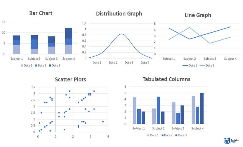
The inspection phase organizes and processes raw data into readable formats and introduces visualizations to illustrate a study’s main points and findings. It’s also where late-stage math is applied to identify and eliminate outliers and generate central tendency figures (i.e., averages). Plotting with calculation can be done by inputting figures into a computer program (e.g., Excel).
Examples of common graphing techniques:
- Bar Charts (e.g., direct subject comparatives)
- Distribution ‘bell’ graphs (e.g., a population’s homogeny or hetero variety)
- Line graphs (e.g., tracking changes over time)
- Scatter plots (e.g., visualizing correlations)
- Tabulated columns (e.g., detailed examinations and ensuring validity)

Measures of central tendency in statistics
Not all relevant numbers are immediately visible in statistics. Figures define where the realistic outer limits of a subject lie and the normal expectations for a set variable.
Central tendency calculations reveal these hidden figures. They serve as good tools for illustrating points and arranging graphs on a sensible scale.
Mean: All factored statistical values are divided by volume (i.e., the average). For example, the mean of the unique range 1-9 is (45/9 = 5).
Median: The value found in the middle of all figures listed from lowest to highest. While the mean and median might be identical, this isn’t always the case due to outliers skewing the mean.
Mode: The most common figure in a variable’s data set. Sum up the occurrence rates and find the most popular figure. More than one mode may occur due to a tie. An entirely diverse sample range (e.g., 1-9) would return p = n for the mode.
Measures of variability in statistics
Measures of variability may also be calculated to indicate how distributed a sample set was from the mean or median and how diverse it was. There are four distinct calculation types:
- Range: The highest set value minus the lowest. E.g., a set with 1-100 at the edges has a range value of 99.
- Interquartile range: The range for the middle 50% of the set. Frequently gives a clear illustration of the most likely variable outcomes.
- Standard deviation: The average (mean) distance of each data point from the set’s overall mean. Also, practical for inferring probable outcomes.
- Variance: Standard deviation, squared.
4. Parameter estimation and hypothesis testing
Testing how well your results match your original hypotheses is the next vital step. If findings are inferred, it may be useful to estimate the full population parameters through data.
Estimation in statistics
Either make a point estimate or an interval estimate from your smaller variable ranges. Choosing a global estimate creates a theory of how the ‘true’ parameter works outside your model.
| Point estimate | Interval estimate |
| • Picks a single integer (i.e. point) as a likely parameter. • This estimate applies to simple, fixed systems with high levels of predictability. Example: When analyzing 1000 coin flips, it can be argued that 0.5 is the exact parameter of a coin landing on either side |
• Applies to data conclusions that are more complex, incomplete, niche, wide-ranging, or experimental. • A range indicates approximately where the parameter variable should be. Example: A 100,000 sample study of coin flips might argue that the interval is 0.49-0.51 due to the faint possibility of a coin landing sideways |
Hypotheses testing in statistics
Running final tests to check how probable the results are within the scope of the null hypothesis are essential steps in statistics.
There are several tests to reach a conclusive comparison. Which type is selected will hinge on the sort of question(s) that are originally asked.
- Comparison testing assesses whether population groupings differed in outcome in standard tests or against different causative factors. Between-subject studies will use these tests first and foremost.
- Correlation testing assesses how well two (or more) values were correlated. Exact causation remains unassessed by design.
- Regression testing assesses causation and connection, demonstrating if X affects Y.
Once you have a final test value (t), it’s measured against your hypothetical null variable to produce a standardized probability (p) value between 0 and 1. If your p-value comes in as >0.05? It’s statistically significant!
You can then make conclusive qualitative judgments on what’s been shown in your study.
Parametric testing
Parametric tests are used for a second-stage check where the collected data follows an inferable, homogeneous standard distribution as evidenced in similar studies. Carefully applying parametric measures to finished sets will help validate the research.
Parametric testing measures predictor variables against known outcomes (i.e., test results). A successful parametric test broadens the data’s applicability.
If the ranged data returned is far outside the assumptions, parametric checks may be employed to ensure that it’s not faulty or anomalous. Non-parametric (random distribution) methods may be relevant to use if a standard distribution can’t be found.
There are four main parametric tests operating:
- Guides and calculators online will simplify each process.
- Realistic estimates to test a hypothetical ‘nominal’ distribution scenario
| Parametric tests | Function |
| Simple linear regression tests | • measure one predictor against one outcome for broad synchronization. |
| Multiple linear regression tests | • measure two or more predictor variables against one outcome for the same. |
| Comparison tests | • check how the variable mean(s) between similar sets and groups roughly match up. • can be applied to different groups within the same test if an outlier appears as a control. • T-value tests cover sample sizes over 30 between one or two values. • Z tests cover all of the above. • ANOVA testing can process three or more group variables at once. |
| Pearson's Correlation | • is a robust formula that establishes whether the same r-value exists in two independently correlative variables. • is practical in meta-studies that collect and analyze results from widely researched fields. |
Printing Your Thesis With BachelorPrint
- High-quality bindings with customizable embossing
- 3D live preview to check your work before ordering
- Free express delivery
Configure your binding now!
5. Concluding in statistics
The final step of every study in statistics is to interpret what can be learned from analyzing the samples by summarizing the results. Postscript analysis may also be applied to aid an understanding and double-check for errors. Moreover, it should give the reader a clear indication of whether the null hypothesis was (dis)proven and to what extent.
Hypothesis significance testing in statistics
The distance of the final p-value from >0.05 (null) determines which broad qualitative interpretation should be provided to the audience and how to proceed.
Lower values suggest there might be great statistical validity and replicability in the findings. A faint result (e.g., 0.048) proposes that better causation and context are needed to infer anything substantial about the topic. High values, closer to 1, indicate the topic is affected in relation to something else than studied.
Type I and II errors in statistics
Statistics may also be prone to unexpected errors. These come in two kinds:
- Type I errors are false positives.
- Type II errors are false negatives.
While rare, both may still have dangerous effects if taken at face value.
A false positive is a fluke result that indicates something demonstrably untrue (e.g., if you take a clinically-proven blood test, there is still a 1% chance it glitches and detects an illness that doesn’t exist).
A false negative is an inverse. Both errors can result from miscalculations, odd sets of harvested data, sensor errors, or poor assumptions (e.g., false causation) that somehow pass the statistical test cycle unscathed.
In many cases, the statistical validity was underpowered, or the initial methodology had unexamined flaws. Applying common sense to the findings and reapplying parametric analysis may help investigate any suspects.
When detecting a Type I or II error, the original study may be re-run with another set and more statistical power. Increasing the sample size, diversity of sampling, and significance threshold may vastly improve the next batch of results.
Overview of all statistics articles
- Akaike information criterion
- ANOVA in r
- Arithmetic mean
- Central tendency
- Chi-square test of independence
- Chi-square tests
- Chi-square distribution
- Chi-square distribution table
- Chi-square goodness of fit test
- Coefficient of determination
- Confidence interval
- Correlation coefficient
- Data outliers
- Descriptive statistics
- Effect size
- Geometric mean
- Inferential statistics
- Interquartile range
- Interval data
- Levels of measurement
- Linear regression in r
- Median
- Missing data
- Mode
- Multiple linear regression
- Nominal data
- Normal distribution
- Null and alternative hypotheses
- One-way ANOVA
- Ordinal data
- Parameter vs. statistic
- Pearson correlation coefficient
- Poisson distribution
- Probability distribution
- Quartiles and quantiles
FAQs
A way of gathering, examining, and presenting numerical, quantitative data from empirical (‘real’) measurements. It helps archive detailed data about a population for future (longitudinal) use and to stress test other’s theoretical assertions.
A fraction of factual, numerical information about a topic derived from sampling a select population. The word statistics derives from ‘status’. Usually, statistics express fixed 0–100 percentages or a regular integer.
Scientists, manufacturers, biomedical researchers, ecologists, mathematicians, political scientists, psephologists (poll predictors), journalists, sociologists, psychologists, market researchers, economists, logistical planners, disaster planners, engineers, computer programmers – and many more professions!
No. A study based on statistics is only a simplified snapshot of how a part of our reality usually behaves. Statistics are distinct from mathematical parameters because they are used to building less detailed ‘scale models’ of a population.