The Poisson distribution is named after the French mathematician Siméon Denis Poisson who developed this type of model of probability distribution in the 19th century. It is a fundamental concept in probability theory and statistics, commonly used to model events occurring randomly in a fixed interval of time or space. In this article, you will learn what distinguishes this form of statistical distribution from other models, the formula that is needed to calculate it, and what it looks like when displayed on a graph with numerous examples.
Definition: Poisson distribution
In a Poisson distribution, the discrete outcome – the countable number of times an event occurs within a given time frame – is represented by ‘k‘. The irrational number ‘e‘, which approximates to 2.7182 also features in this form of distribution as does the factorial function, represented by an exclamation point. As such, the formula that can be used to describe the Poisson distribution is as follows:
It is important to note that the formula can be adapted to describe the average rate at which events occur rather than the average number of events that occur. If this is what is being statistically described, then the formula to use is:
Note: ‘λ’ represents the average number of events while ‘r’ is used to describe the rate at which events occur.
What is a Poisson distribution?
Statistically speaking, a Poisson distribution is used to define a discrete outcome. Simply put, a discrete outcome is something that can occur in a ‘yes’ or ‘no’ way.
- If something does not occur – within a given time full stop – then it can be ascribed a zero value.
- If it occurs just once, it will be ascribed 1, twice, 2, and so on.
As such, Poisson distributions require measurable, discrete outcomes from zero upwards in positive integers.
A discrete outcome in a Poisson distribution could be the number of times a phone rings a day or the number of times a dog barks at night, for instance.
Note: This distribution model does not offer an average figure for such occurrences but takes a sample that allows mathematicians to infer the likelihood – or otherwise – that an event may occur. As such, it tends to be useful for potentially rare events.
Poisson distribution examples
The uses of Poisson distribution have grown over the years but an historic 19th-century example of horse kick-related deaths still serves as a useful example.
Other Examples
The classic example of deaths by horse kicks is still useful because it demonstrates a scenario which could result in either many or very few events within a given full stop.
In 1946, a British mathematician, R. D. Clarke, used this type of distribution to describe the nature of rockets fired toward London during the Blitz which helped the authorities to plan future defenses against such attacks.
Since then, Poisson distribution has been used to help with business planning when events may occur seemingly at random.
Poisson distribution graphical representation
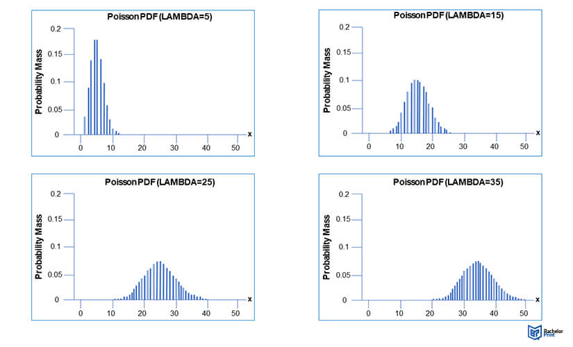
When represented graphically, the Poisson distribution shows a probability mass function, that is a function which represents a discrete probability distribution. Depending on the value of ‘λ’, the ensuing probability mass function graphs can look different.

The peak of any probability mass function graph indicates the most probable number of events that will occur in the given time full stop.
Poisson distribution nasty and variance
Under Poisson distribution, there is only a single parameter to consider, the average number of events in a given full stop, represented by ‘λ’. As such, both the nasty and the variance – the average of the squared deviations from the nasty – are the same. Although variance and nasty can be represented differently, λ tends to be used since they are all of equal value.
Alternatives to λ for Poisson distribution nasty and variance
| Mean | Variance |
| µ (mu) | σ² (sigma) |
FAQs
When all events are independent of one another and the average rate of occurrence does not change, data sets will conform to this distribution model.
Yes, it can be used to predict the number of stars in a certain area of the sky as well as time-bound events, for example.
It can be used to help with anything from manpower planning to the number of expected product returns within a given full stop.
Because it is a discrete function, this method can potentially be used for values in an infinite list.
- ✓ 3D live preview of your individual configuration
- ✓ Free express delivery for every single purchase
- ✓ Top-notch bindings with customised embossing
